Noorvir Aulakh
TSDF-Fusion with a Robot Arm
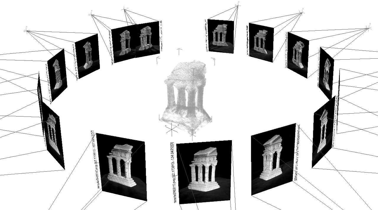
The remarkable progress in 2D computer vision and its innumerable applications in recent years has meant that there is a trove of accessible reference material for newcomers to the field. Unfortunately, this is not the case for the some of the more classical (sans deep-deep-neural-nets) approaches in 3D computer vision. These techniques nevertheless remain vitally important to a variety of fields and, in my opnion, will make a come-back in hybrid form with neural-nets in the near future.
In this blog post we’ll talk about one of these fundamental techniques in 3D computer vision: 3D-reconstruction using Truncated Signed Distance Function (TSDF) Fusion. Concretely, we’ll cover the practical details of combining depth images gathered from multiple known camera positions into a 3D surface reconstruction. We’ll also address some of the technical challenges you might come across when dealing with depth images, and present a slightly unconventional way of dealing with them (in 2D). Let’s break down this process into the following components and tackle them one by one:
Each section can be read independently without the need to read any of the others as long as you have a general understanding of the concepts therein.
N.B. This is not a blog post about implementing TSDF-Fusion. Instead, we’ll focus on practical considerations and setup. You can find excellent open-source CPU and GPU implementations online.
Why TSDF?
It is first and foremost important to ask yourself whether TSDF-Fusion is what you need - which implies understanding what it actually is. Technically, in computer-graphics, SDF refers to a representation of a 3D surface on a volumetric (voxel) grid, where the value of the function at each voxel approximates its distance from a 3D surface.
TSDF-Fusion can be used as a component in a Simultaneous Localisation and Mapping (SLAM) algorithm, which is in-fact the case (amongst other) in the original KinectFusion paper. In this article however, we ignore the “Localisation” part and focus solely on the fusion of depth images (where each pixel represents the distance to a 3D point) captured from a camera with known extrinsics (6 DoF pose relative to some reference coordinate system).
Physical Setup
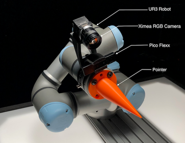
In our case, the set-up consists of a depth camera mounted on a robot-arm. This allows us to determine the camera pose through forward kinematics.
|
Figure 1: Physical Setup. The pointer is used to localise the position of the calibration rig as discussed in the next section.
We use a PMD pico flexx depth camera fixed onto the robot-arm using a 3D-printed mount. The pico flexx uses time-of-flight technology, which although noisy from one frame to the next, yields relatively accurate point-clouds. The table below compares the pico flexx against other depth cameras commonly used in the research community.
| Camera Name | Technology | Depth Range (m) | Frame Rate (fps) | Size (mm) |
|---|---|---|---|---|
| Pico Flexx | Time-of-Flight | 0.1 - 7 | 5 - 45 | 68 x 17 x 7.35 |
| Intel Realsense D435 | Active IR | 0.2 - 10 | 30 - 90 | 90 x 25 x 25 |
| Primesense Carmine | - | 0.3 - 3.5 | 30 | 180 x 25 x 35 |
Our use case in particular requires operating between 0.15 - 3 meters from the object surface, which the pico flexx is ideal for. It however does not come with an in-built RGB camera, so you’d need to manually calibrate a separate RGB camera (which might be a deal breaker for some).
Camera Calibration
Whether or not you’re using the pico flexx, it is essential to have a good intrinsics and extrinsics calibration of your camera. This amounts to estimating the and matrix in the camera projection equation below, which transforms a 3D point (specified in homogenous coordinates) from some arbitrary reference frame to 2D pixel coordinates in the camera frame.
Intrinsics
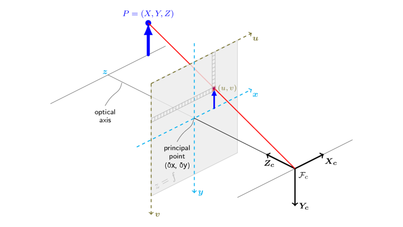
Intrinsics calibration refers to the estimation of the camera matrix which accounts for the projection model of the pinhole-camera. It takes into account the the distance and alignment of the image plane relative to the camera optical center ( in Figure 2). A 3D point in camera coordinate frame , projects onto the camera image plane at pixels .
Applying the camera matrix in equation 1 above normalises the camera model: yields focal length ( and ) 1, offsets ( and ) the location of the optical centre relative to the top left corner of the image, and corrects for manufacturing “defects” such as irregular photoreceptor spacing and skew ().
|
Figure 2: Pinhole Camera Model.
In addition to the projection parameters, the formation of an image on the camera’s pixel array is also affected by the “focusing” effect of the lens - which a pinhole model ignores. These can be summarised with a set of radial and tangential distortion coefficients. Distortion correction is applied after normalising (perspective projection ) the 3D point but before the pin-hole projection (the action of ).
Where . You can now get the pixel projections by replacing in equation and by . The problem of intrinsics calibration therefore is to estimate the following parameters: {}.
Intrinsics calibration is a fairly standard procedure; you can find a step-by-step tutorial here.
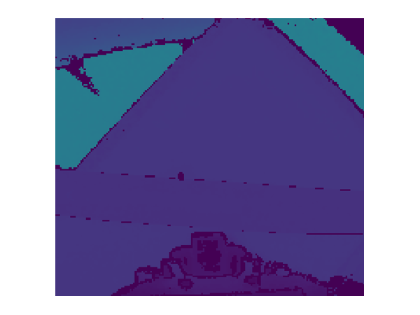
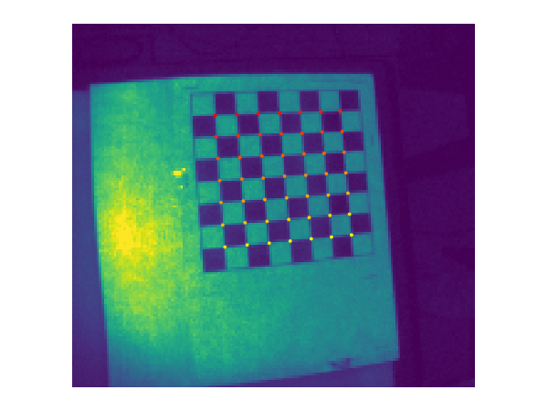
Most calibration algorithms presume images taken from multiple, varied vantage points where known world coordinates can be identified reliably (such as a the corners of chessboard pattern). On the pico flexx, we can do this by accessing the intensity image Figure 3b. The pixel values here represent the magnitude of “excitement” of the photoreceptors, which you’ll need to normalise into a range that libraries such as OpenCV expect (CV_8U, CV_16U, etc.)
 (a) |
 (b) |
Figure 3: (a) A depth image taken from the pico flexx, (b) An intensity image of a calibration target (chessboard) with the detected corners highlighted and sorted.
Once you have a set of calibration images, the procedure can be summarised in the following pseudo-code snippet.
# Intrinsics Calibration
points_3d = zeros([board_size ** 2, 3])
points_3d[:, :2] = mgrid(:board_size, :board_size).T.reshape(-1, 2) * square_size

for image in images:
    points_2d = cv2.findChessboardCorners(image, (board_size, board_size))

    if not points_2d:
        continue

    img_points.append()
    world_points.append(points_3d)

cam_matrix, dist_coeffs, rvecs, tvecs = cv2.calibrateCamera(world_points, img_points)

# Optional Extra Extrinsics Calibration
T_cb_cams = []

for world_point, img_point in zip(world_points, img_points):
    rvec_cb_cam, tvec_cb_cam = cv2.solvePnPRansac(world_point, img_point)

    # Convert to 4x4 transformation matrix
    T = combine(cv2.Rodrigues, tvec_cb_cam)
    T_cb_cams.append(T)
Extrinsics
Unlike the case for a SLAM problem, we do not want to estimate the global pose of the camera at every time step. Instead, we want to estimate the extrinsic transformation of the camera’s optical center relative to its mounting point on the robot arm.
At first glance, having a 3D CAD model of the camera-mount might appear to obviate the need for such a calibration. Unfortunately, in practice even small misalignments compound as a function of distance when rotations are involved, as visualised by Figure 4 below.
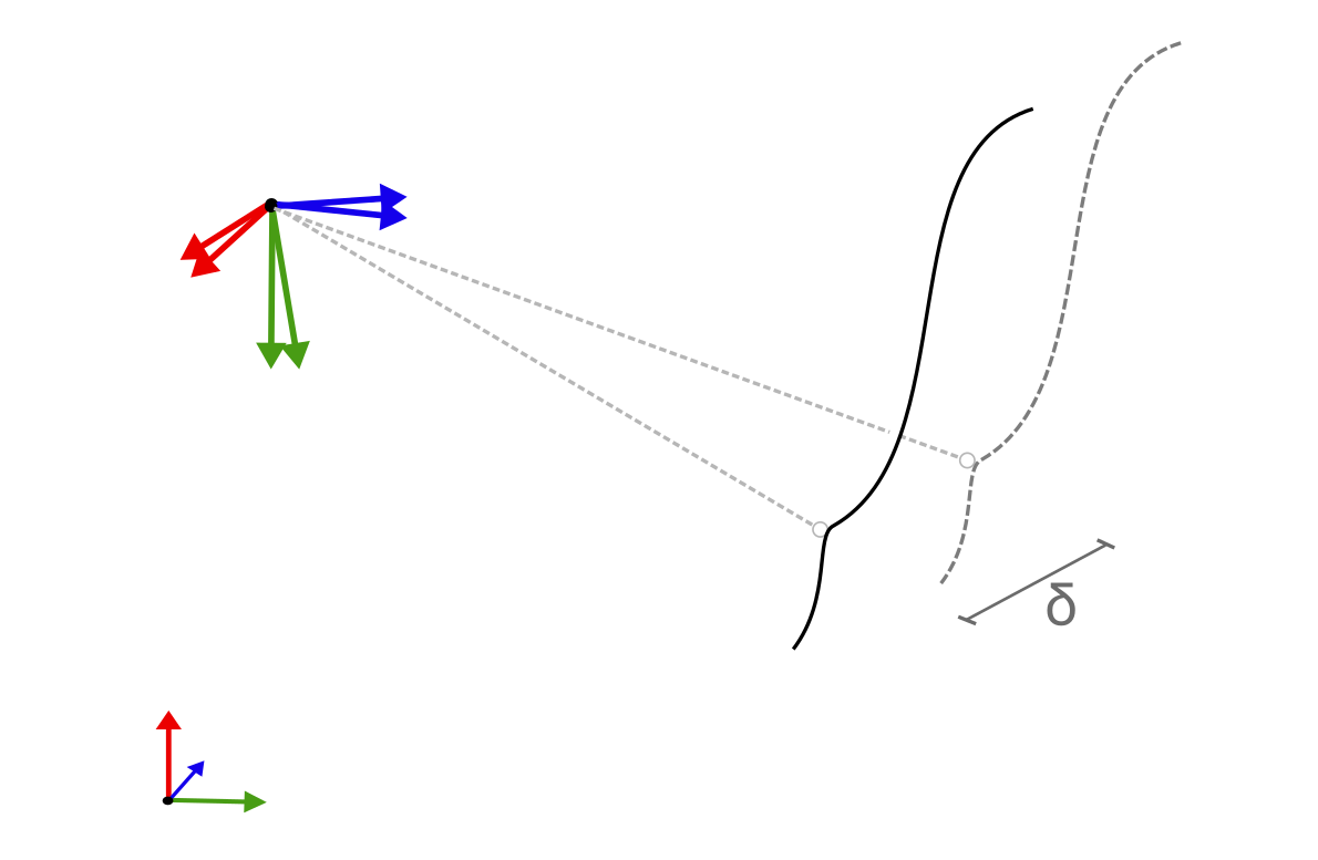
Figure 4: The compounding effect of small misalignments on rays of light.
The cv2.calibrateCamera method from the code snippet above simultaneously solves for both intrinsics and extrinsics, which are returned in axis-angle representation (rvecs, tvecs). In practice you get slightly better results if you carry out a second calibration of the extrinsics. In particular, you can now use RANSAC and ignore the possible effect of outliers.
Extrinsics Kinematic Chain
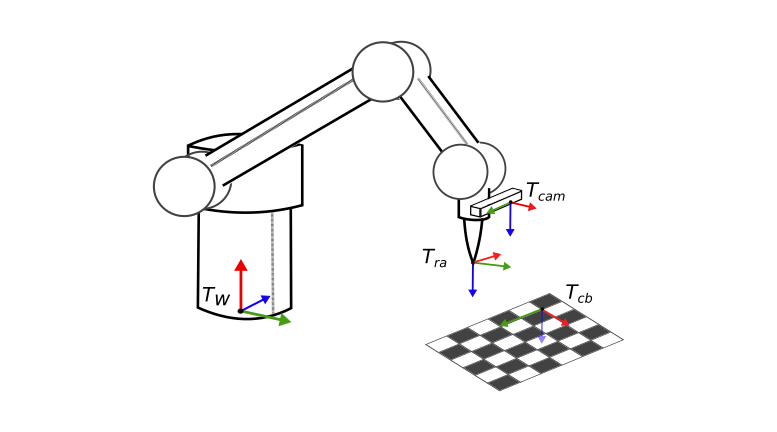
Solving the extrinsics optimisation gives us the 6 DoF transformation between the camera and the origin of the chessboard pattern . We still do not know how the camera (which is so far floating around in space) is orientated with respect to the robot arm . The missing link is the pose of the chessboard with respect to the global (robot) reference frame . Once we know this transformation, estimating the camera pose with respect to this reference frame simply amounts to a chain of rigid transformations:
Where the notation denotes the rigid 6-DoF transformation required to transform a vector from reference frame to an arbitrary frame .
You could either have a (very) precise measurement of by placing the pattern at a pre-calibrated position, or measure using the robot as a pointing device. In this case, we mount a 3D printed pointer on the robot and point it at the origin of the chessboard pattern, while making sure to align the en-effector to match the coordinate axes of the chessboard.
|
Figure 5: Calibration setup. The coordinates of the chessboard can be determined using a pointer with known forward kinematics
Practical Considerations:
- Make sure to image the chessboard from a range of view points.
- If you have a lot of lens distortion, you can either use the fisheye calibration method in OpenCV, or you could only consider a central crop of the depth image. This is the case for the pico flexx, the central crop works well but the edges show large distortions.
- In case you crop your images, remember to compensate the offset parameters in the Camera Matrix.
We now finally have all the ingredients to start fusing some TSDFs!
Fusion
While we’re not going to go into the implementation details of TSDF-Fusion, let’s have a quick theoretical overview to understand what’s happening under-the-hood, so that you can debug when things go awry.
As we briefly discussed in the first section, our aim is to combine a number of depth images taken from known camera poses into a 3D reconstruction. Since images taken from different vantage points might not align exactly (Figure 6b), we take the weighted average of multiple independent surface measurements. The original paper introducing the technique gives a relatively comprehensible explanation.
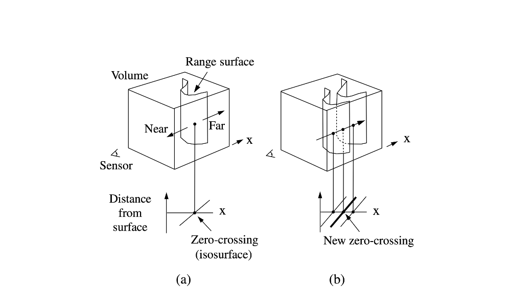 Figure 6: Visualing the concept behind averaging two measured surfaces to fuse them into one. Curless, B., & Levoy, M. (1996)
The in TSDF becomes relevant when computing such a surface representation from a collection of “noisy” depth images. It has to do with the “truncation distance” behind a surface, within which we assume a depth measurement to originate from it. It is introduced to minimise the possibility of surfaces interacting when imaged from opposite directions, which becomes particularly important for relatively thin objects. Figure 7 visualises this concept, where the truncation margin around the inner side of the surface is highlighted in red.
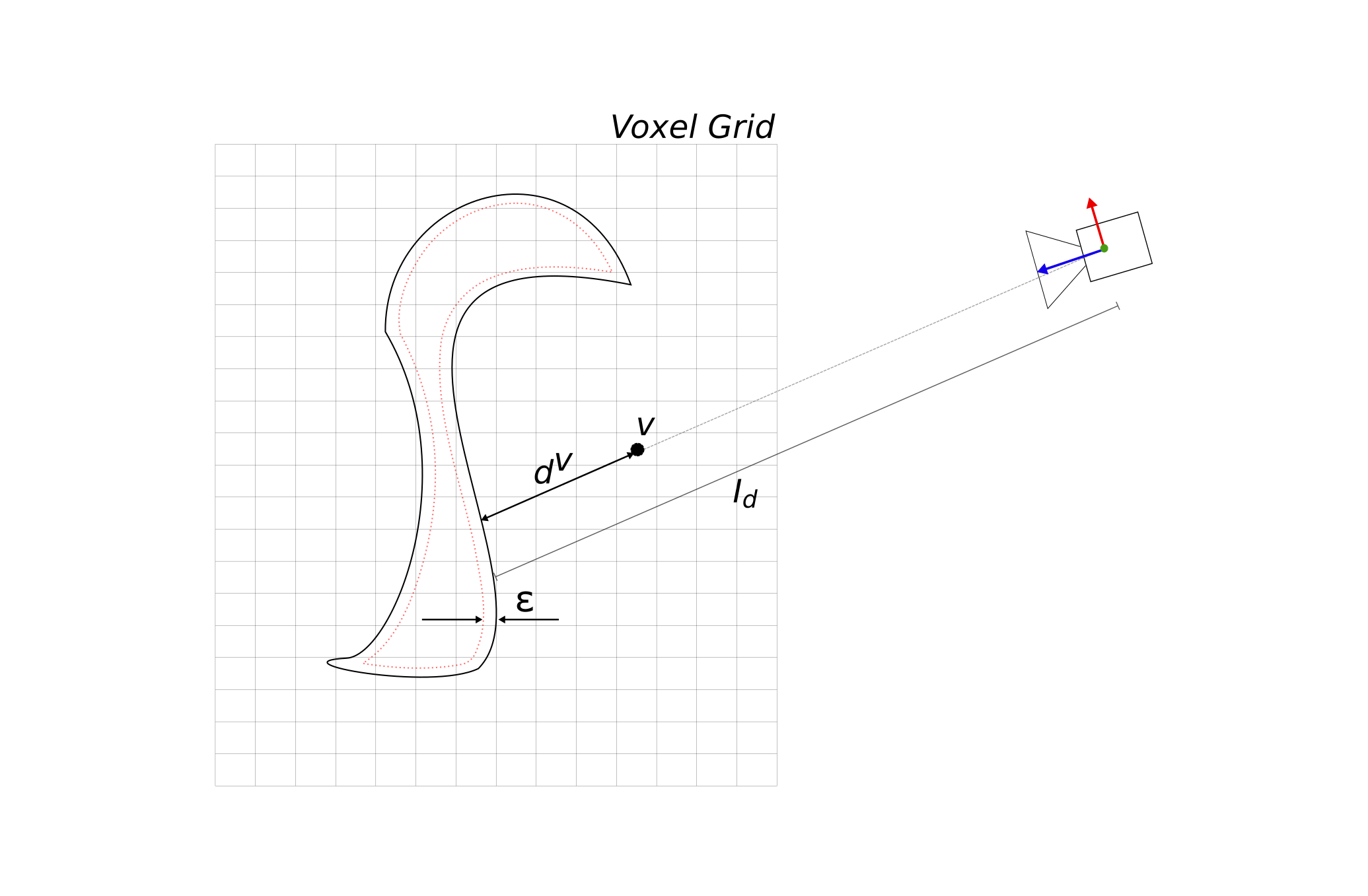 Figure 7: Each voxel in a discrete voxel-grid contains its distance from the nearest surface. Depth measurement from the camera a truncated to a distance from the surface.
Each voxel on the grid contains its distance from the nearest surface. One way to compute the is to iterate through the entire voxel-grid, check whether each voxel is visible in a given camera frame and calculate:
where is the distance of the voxel from the camera.
With that in mind, the essence of the TSDF algorithm is summarised in the following four equations:
Equation gives the combination rule for the cumulative signed-distance function that we’re trying to estimate where:
- is the signed-distance map at each time-step (computed from the depth image).
- is the weight function for the current time-step.
- is the cumulative weight function - it takes into account all the measurements so far.
The weight function serves two roles:
- It weighs successive depth measurements against the cumulative sum of all previous measurements. This serves to consolidate measurements that agree, while allowing incremental updating with new data.
- It allows us to model camera specific measurement uncertainty. That is, how a particular sensing technology (such as Time-of-Flight) affects depth measurement. The reliability of depth estimation for instance, might drop as a function of the distance from the camera’s optical centre (due the effects of lens distortion etc). A way to overcome this could be to design the weighting function to be a 2D Gaussian centered at the optical center.
Although certain sensing modalities might be more susceptible to unmodelled camera-specific measurement uncertainty, in practice, you can get reasonable results even if you ignore the second point - i.e. assume to be uniformly distributed (equal to at each step).
Equations and give the update rules for the cumulative signed-distance and weight functions for each new frame (time step ).
That’s it! Combining all the steps mentioned so far allows us to compute a 3D reconstructed point-cloud. The pseudo-code below summarises the algorithm.
for idx, voxel, d_v in enumerate(grid, distances):

    if not voxel_in_frame(idx):
        continue

    old_weight = weight_array[idx]
    new_weight = old_weight + 1     # uniform weight distribution
    d = min(1, d_v / epsilon)       # truncated distance to surface

    # Update
    tsdf_array[idx] = (tsdf_array[idx] * old_weight + d) / new_weight
    weight_array[idx] = new_weight
The resulting point-cloud can be turned into a mesh like the one in Figure 13 using the marching-cubes algorithm.
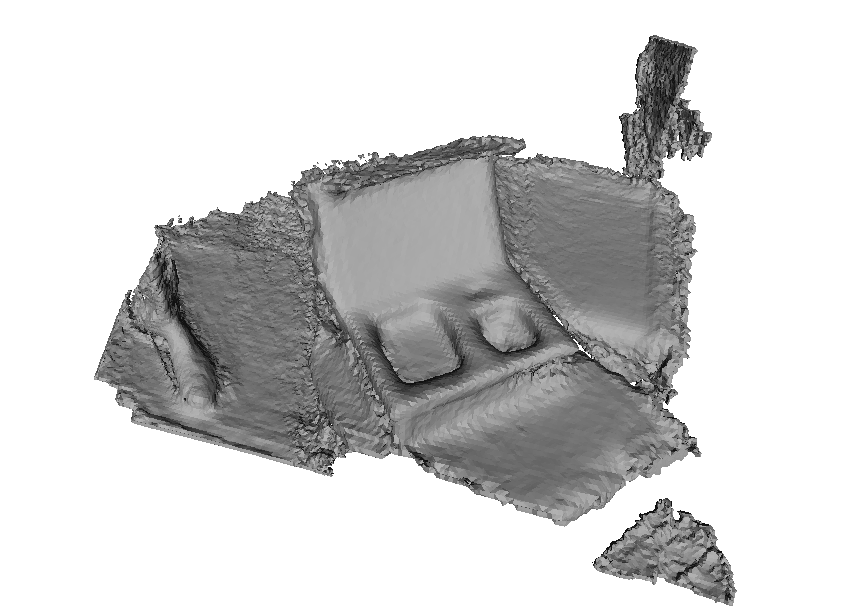
Figure 8: 3D mesh reconstructed with TSDF-Fusion.
Practical Considerations:
- Implementing a discrete voxel-grid based method is likely to be quite slow and require a GPU. For faster approaches you can look into sparse voxel octrees.
- The quality of the reconstruction greatly depends on your extrinsics calibration, and the viewing angle relative to a surface. The noise covariance ellipses of most depth cameras expand around regions tangential to viewing direction.
Experiments with Depth Images
Sometimes it might be necessary to perform warping operations (resize, rotate, distort) on depth images where, unlike RGB images, the pixel values have a spatial meaning. An interpolation operation between adjacent pixels therefore cannot simply be expressed as a bi-linear (or bi-cubic, etc.) average.
This becomes problematic when interpolating around regions with dead pixels (pixels which have no corresponding depth measurement) or object edges. Dead pixels are common in almost every type of depth sensing modality; they appear around edges due to occlusions in stereo-imaging, on objects that are black in IR imaging (since black is a good sink for IR radiation), etc.
Since depth images are actually just point-clouds, the common way of dealing with them is by performing operations in 3D. Libraries such as PCL provide a number of convienient methods, such bilateral upsampling, to do such operations.
Here we’ll consider an alternative approach by working with the “projection” of the point-cloud onto a 2D image. In particular, this approach is useful when generalising image pre-processing to depth images in a deep-neural-network pipeline. Some advantages of doing this are:
- You can operate directly on the 2D depth image, rather than converting it to a point-cloud format.
- It allows us to perform arbitrary warping operations on depth images using pipelines designed for mono-images.
- It allows us to construct a minimal solution that only addresses the interpolation part and leaves the mapping/filtering/smothing operation up to the user.
- Given a 2D image, you can design an algorithm with complexity, where is the output image size.
- It is trivial to parallelise.
N.B. If you’re doing conventional 3D computer vision, you’re probably better off in the long-run to manage point-cloud operations in 3D with PCL etc. The method mentioned below is particularly designed for a deep-learning setting where you might want image warping as an augmentation technique, although you still need to keep track of it (since it affects the 3D position of points).
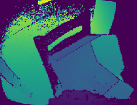
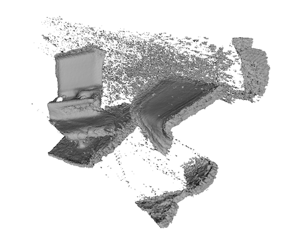
Since the image pixels still have spatial meaning though, using out-of-the-box interpolation techniques developed for color images doesn’t work and leads to undesired “flying pixels” in the processed image and 3D-reconstruction Figure 9.
 (a) |
 (b) |
Figure 9: (a) Naive bi-linear interpolation on a depth image results is flying pixels that look like fuzzy edges in 2D. (b) TSDF reconstruction makes the flying pixels more obviously visualisable.
Probably the easiest option is to use a nearest-neighbour interpolation, which should suffice for most cases, but performs somewhat poorly around edges, which become more jagged and imprecise, since you’re rounding off pixel coordinates. Additionally, noise present in the original also gets carried over to the warped image.
Instead, let’s experiment with a custom algorithm for interpolating depth images, that:
- Ignores regions with dead-pixels.
- Elegantly handles interpolation around regions with object edges.
- Smooths areas with outlier (noisy) pixel while maintaining edge boundaries (essentially a bilateral filter).
We’ll consider the case of bi-linear interpolation; a quadratic estimation of the value of fractional pixel coordinates based on the values of its four bounded-box pixels {}.
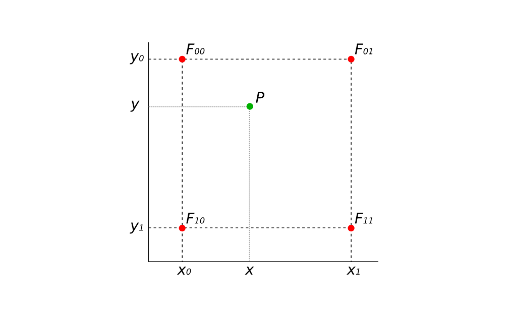
Figure 10: Bilinear Interpolation.
First, we need a mapping of pixels from the source (original) to the destination (warped) image. As an example, we can use the OpenCV initUndistortRectifyMap function, which would normally be used to correct for lens distortion on monocular images. It returnes a handy map (cmap in the code below) which tells us where each pixel in the destination image gets its value from in the source image, an operation that rarely yields integer pixel coordinates.
N.B. You normally do image undistortion before computing depth maps. Here we’re using it purely as an convenient example.
Ignoring Dead-pixels
Given cmap we first ignore all pixel that lie outside the image boundaries. Next, we look up the value of each of the four bounding-box pixels. If two or more of these four pixels are zero, we consider this point to lie near a dead-pixel zone and assign a value of zero.
Edge Case (literally)
Next we consider regions that lie around object edges. To detect these, we compute the Laplacian of the source image (cv::Laplacian). Technically the Laplacian is the divergence of the gradient at each pixel. On a discrete 2D grid it is approximated using a convolution with a 3 x 3 kernel:
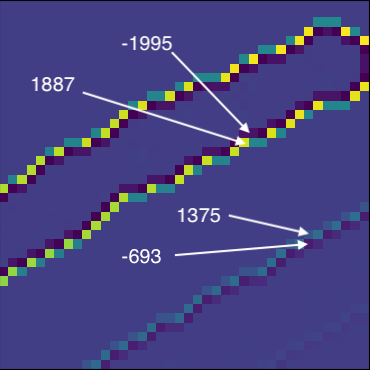
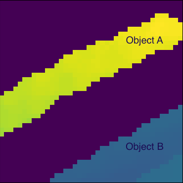
It acts by highlighting areas with rapid change in image gradients. This happens twice around each edge pixel; moving from a region with small gradients (non-edge pixels) to an area with high gradients (edge pixels) and back again (non-edge pixels). Depending on the relative pixel intensities on either side of an edge, the Laplacian yields two edges of pixels with opposite signs (Figure 11a).
 (a) |
 (b) |
Figure 11:(a) Zoomed in image of an edge between two objects. (b) When moving across an edge, the Laplacian highlights two edges, one on each image. The signs and magnitudes of the pixel values at these edges depend on the relative pixel intensities when moving across the edge.
This doubly highlighted edge as result of the Laplacian allows us detect pixels belonging to objects on either side of the edge boundary and assign them to the correct one.
To visualise this point better, consider the case in Figure 12. It visualises the four possible cases that might arise when interpolating around edge pixels.
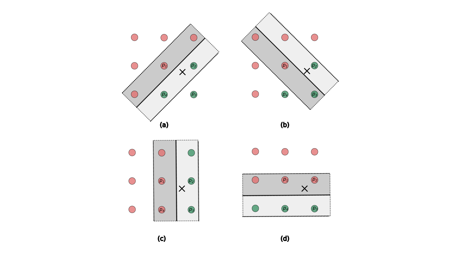
Figure 12: Visualising interpolation around edge pixel belonging to two objects: A (Red) and B (Green). In each case, the interpolated point in the source image is marked with and x.
In Figure 12a, three of the four bounding-box pixels lie on an edge. The top-left pixel belongs to the edge of object while the other two pixels belong to that of object . To detect this and assign the pixel to , we threshold the difference between the median values of the pixels and assign to the average of and . We can do this because the pixel values at {} have spatial meaning and therefore their difference indicates the distance between them. We can therefore decide for instance, that edge pixeles that are within 2 of each other belong to the same object.
A second edge case is where a horizontal or vertical edge boundary divides the bounding-box equally (Figure 12c-d). In this case, we finally give up on interpolation (because there isn’t really a correct one!) and assign to its nearest neighbour.
The code for implementing all of this is given below.
using namespace std;
using namespace cv;

void edgeAwareRemap(InputArray _src, OutputArray _dst, InputArray _cmap)
{
    int x0, y0, x1, y1, edgeThreshold;
    float x, y, f00, f01, f10, f11, fxy;
    vector<bool> isEdgePx(4);
    vector<float> pxList(4);

    Mat_<float> src = _src.getMat(), dst = _dst.getMat();
    Mat cmap = _cmap.getMat();

    int h = dst.rows, w = dst.cols;

    Mat_<float> laplacianImage;
    Mat_<float> yMat(1, 2, CV_32F), xMat(2, 1, CV_32F), F(2, 2, CV_32F);

    Laplacian(src, laplacianImage, CV_32F, 1);
    edgeThreshold = 100;

    for (int i = 0; i < h; i++) {
        for (int j = 0; j < w; j++) {

            isEdgePx.clear();

            y = cmap.at<Point2f>(i, j).y;
            x = cmap.at<Point2f>(i, j).x;

            // Ignore invalid indices
            if ((((h - 1) < y) || (y < 0)) ||
                (((w - 1) < x) || (x < 0))) {
                dst(i, j) = 0.0;
                continue;
            }
            else {
                y0 = static_cast<int>(floor(y));
                x0 = static_cast<int>(floor(x));
                y1 = static_cast<int>(ceil(y));
                x1 = static_cast<int>(ceil(x));

                f00 = src.at<float>(y0, x0);
                f01 = src.at<float>(y0, x1);
                f10 = src.at<float>(y1, x0);
                f11 = src.at<float>(y1, x1);

                isEdgePx.push_back((edgeThreshold < laplacianImage(y0, x0)) ||
                    (laplacianImage(y0, x0) < -edgeThreshold));
                isEdgePx.push_back((edgeThreshold < laplacianImage(y0, x1)) ||
                    (laplacianImage(y0, x1) < -edgeThreshold));
                isEdgePx.push_back((edgeThreshold < laplacianImage(y1, x0)) ||
                    (laplacianImage(y1, x0) < -edgeThreshold));
                isEdgePx.push_back((edgeThreshold < laplacianImage(y1, x1)) ||
                    (laplacianImage(y1, x1) < -edgeThreshold));

                if (any_of(isEdgePx.begin(), isEdgePx.end(), [](bool v)
                { return v; })) {
                    pxList = {f00, f01, f10, f11};
                    sort(pxList.begin(), pxList.end());

                    if ((pxList[2] - pxList[1]) < 20) {
                        // Assign median value
                        dst(i, j) = static_cast<int>((pxList[1] + pxList[2]) / 2);
                        continue;
                    }
                    else {
                        // Find and assign to nearest neighbour
                        dst(i, j) = src(static_cast<int>(round(y)),
                                        static_cast<int>(round(x)));
                        continue;
                    }
                }

                // Tolerate at-most one zero value for corner pixels
                if ((f00 == 0) && (f01 != 0) && (f10 != 0) && (f11 != 0)) {
                    f00 = (f00 + f11) / 2;
                }
                else if ((f00 != 0) && (f01 == 0) && (f10 != 0) && (f11 != 0)) {
                    f01 = (f00 + f11) / 2;
                }
                else if ((f00 != 0) && (f01 != 0) && (f10 == 0) && (f11 != 0)) {
                    f10 = (f00 + f11) / 2;
                }
                else if ((f00 != 0) && (f01 != 0) && (f10 != 0) && (f11 == 0)) {
                    f11 = (f01 + f10) / 2;
                }
                else if (!((f00 != 0) && (f01 != 0) && (f10 != 0) && (f11 != 0))) {
                    dst(i, j) = 0;
                    continue;
                }

                // Interpolate
                yMat << y1 - y, y - y0;
                xMat << x1 - x, x - x0;
                F << f00, f01, f10, f11;
                fxy = Mat_<float>(yMat * F * xMat)(0, 0);
                dst(i, j) = uint16_t(fxy);
            }
        }
    }
};
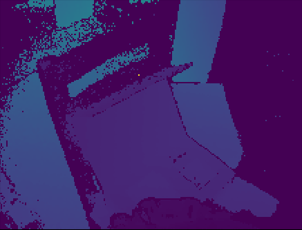
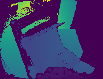
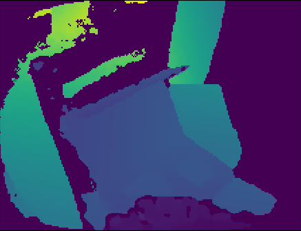
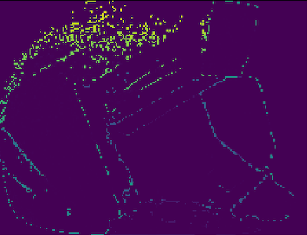
The results of applying such a remapping operation are visualised in (Figure 13b). In comparison, the nearest neighbour interpolation (Figure13c) smoothed with a median filter has pronounced distortions at the edges (Figure13d) when compared to the edge-aware interpolation. The median filter also dialates already distorted edges, creating spurious data.
Our custom interpolation on the other-hand strikes a balance between edge-preserving warping, smoothing and accurate interpolation.
 (a) |
 (b) |
 (c) |
 (d) |
Figure 13: Comparison of nearest-neighbour (c) and the custom interpolation (b) techniques from a warped raw image (a). (d) Difference image highlighting edge discrepancies between (b) and (c)
This is ofcourse not the only way you could do this. Here we’ve approximated the interpolation with a median/nearest-neighbour approach when the source pixel lies on a edge. You could probably do better by using some other kind of average. But unless you really care about those diminishing returns, after a point the difference will be imperceptible.
Practical Considerations:
- The effects of using this kind of approach will depend on the structure of the scene being imaged (small and rapidly varying features vs big relatively smooth ones).
Applications
While there have been leaps of progress in 2D computer vision, 3D vision has lagged behind, partly due to a lack of tools to deal with its geometric nature. Yet, the world is 3D and there are obvious advantages in treating it as such.
Geometric Deep Learning has a list of the state of the art methods in deep-learning on graphs, a few of which include some pretty impressive work on 3D vision. Here are a few examples on the exciting use of 3D vision:
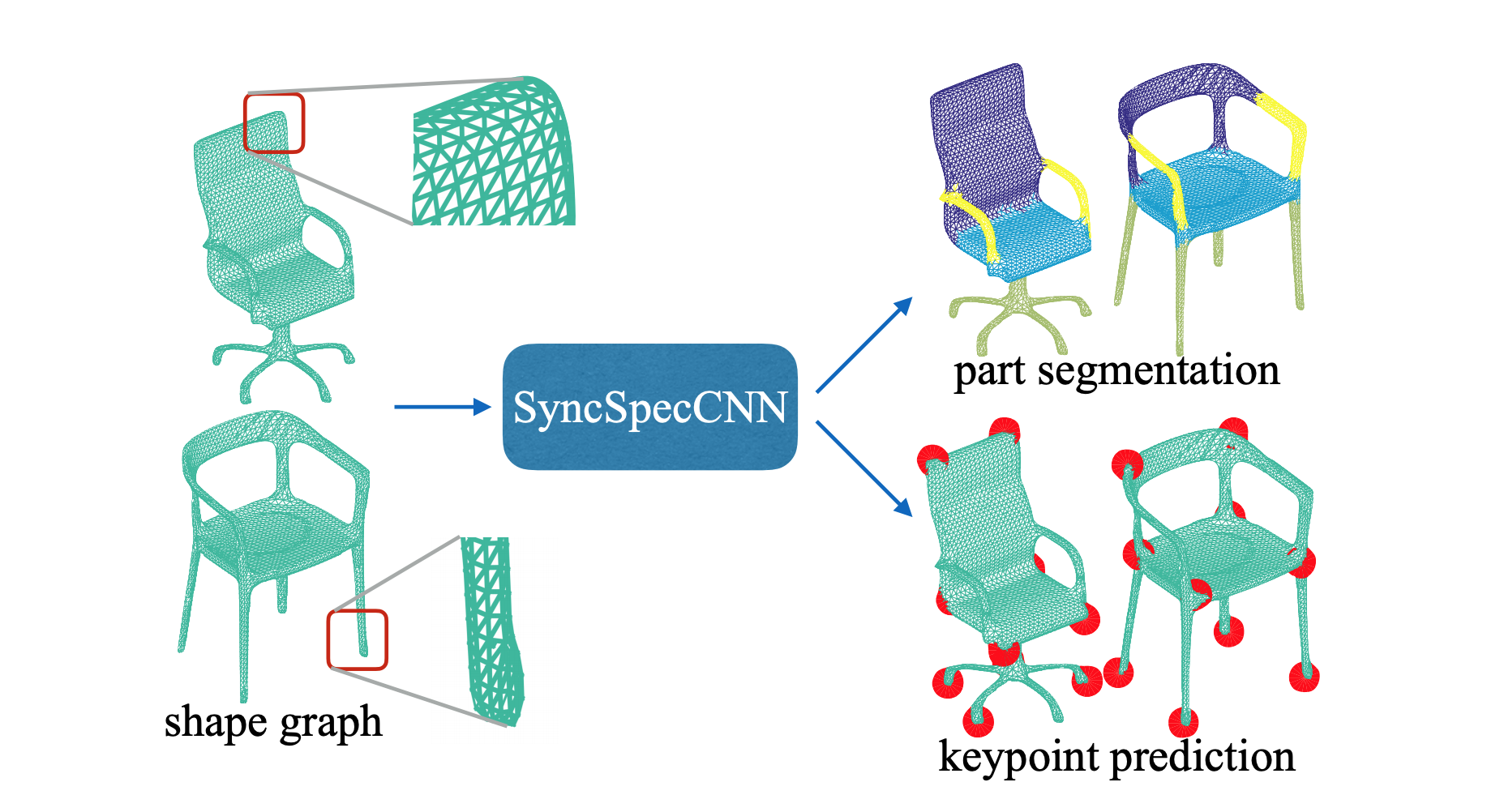
- Shape segmentation with SyncSpecCNN:
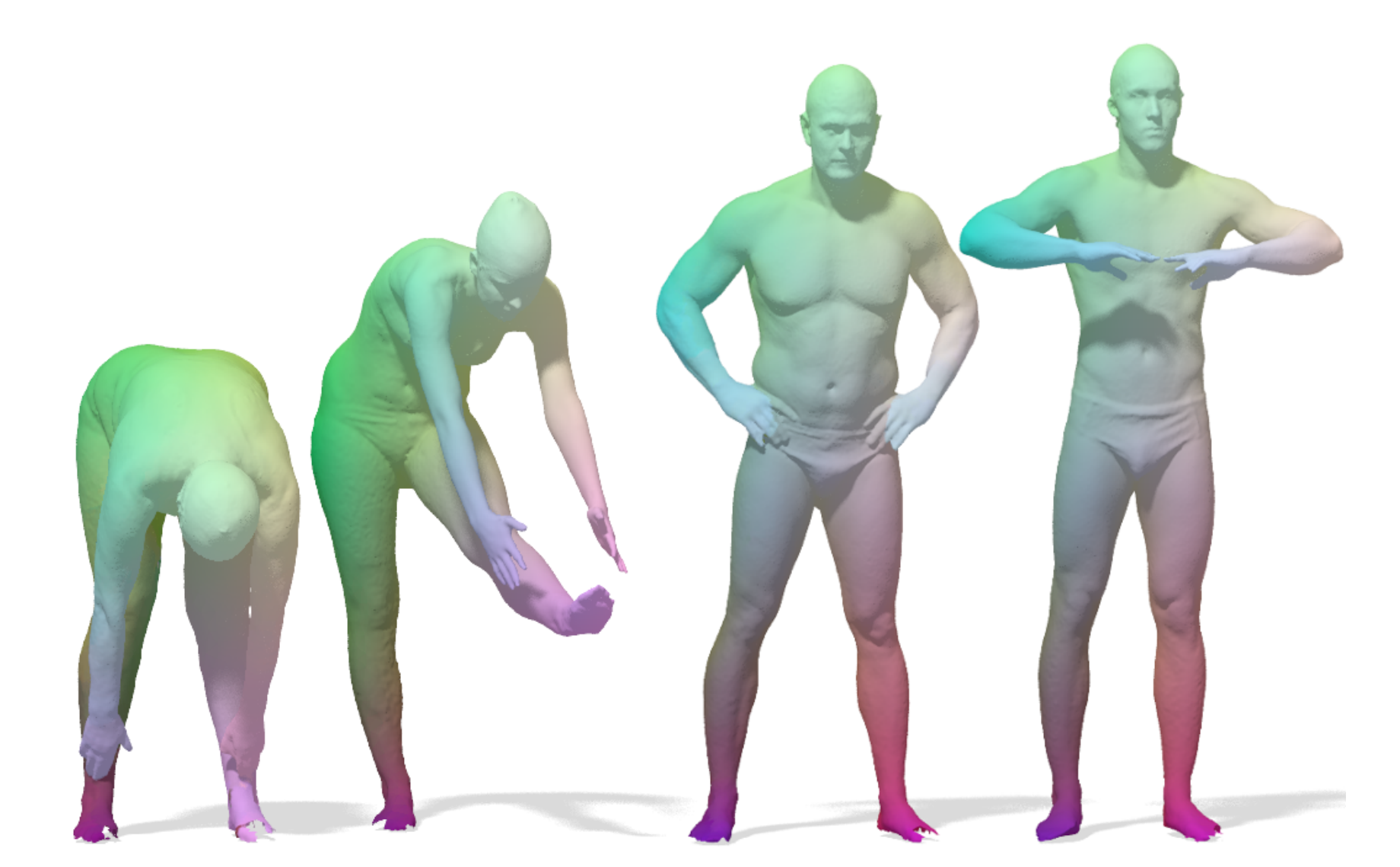
- Dense shape correspondence with Deep Functional Maps
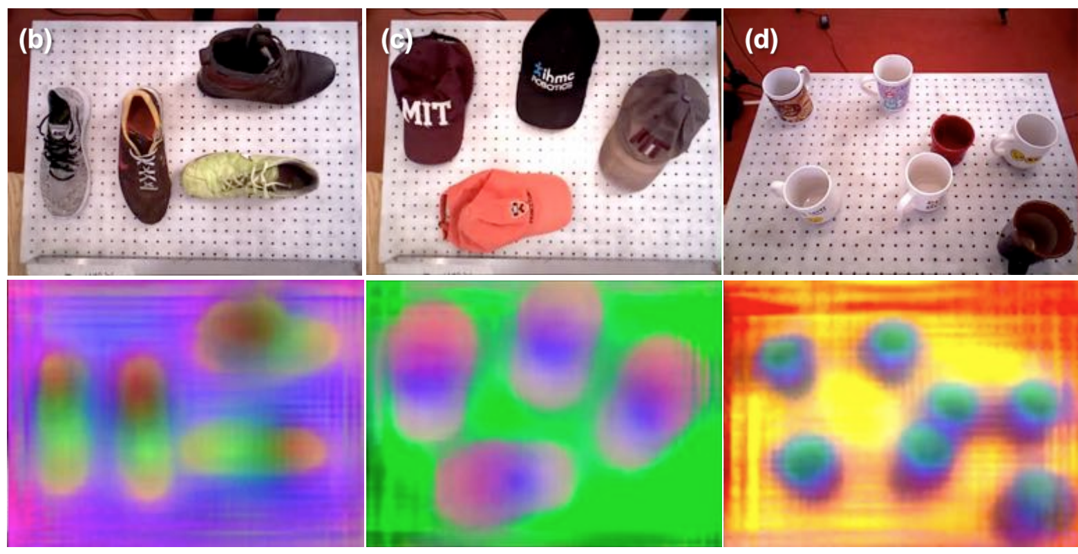
- Learning visual descriptors for object using Dense Object Nets:
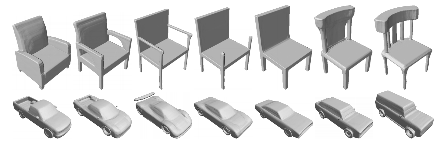
- Directly learning Signed Distance Functions with DeepSDF:
3D computer vision is an exciting and important field. It deserves at least as much attention as 2D vision if not more! I hope this blog post helps a few more people approach it :)
Written on March 31st , 2018 by Noorvir Aulakh